43 excel data labels from third column
Mac Excel 2008 - How to add Data Labels for Scatter Plot coming from ... In Excel 2008, to select X axis for the labels: go to 'Formatting palette' navigate to 'Chart Option' Under 'Other options' select "category name' in Labels. A AsherS New Member Joined Feb 9, 2012 Messages 9 Jul 30, 2014 #3 Cyrilbrd, this does not add a label from another column. This only displays the X-value and does not solve the issue. cyrilbrd Custom data labels in a chart - Get Digital Help You can easily change data labels in a chart. Select a single data label and enter a reference to a cell in the formula bar. You can also edit data labels, one by one, on the chart. With many data labels, the task becomes quickly boring and time-consuming. But wait, there is a third option using a duplicate series on a secondary axis.
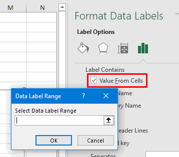
Add or remove data labels in a chart - support.microsoft.com Right-click the data series or data label to display more data for, and then click Format Data Labels. Click Label Options and under Label Contains, select the Values From Cells checkbox. When the Data Label Range dialog box appears, go back to the spreadsheet and select the range for which you want the cell values to display as data labels.
Excel data labels from third column
3 Axis Graph Excel Method: Add a Third Y-Axis - EngineerExcel Create a 3 Axis Graph in Excel. Scale the Data for an Excel Graph with 3 Variables. Decide on a Position for the Third Y-Axis. Select the Data for the 3 Axis Graph in Excel. Create Three Arrays for the 3-Axis Chart. How to Add a Third Axis in Excel: Create an "axis" from the fourth data series. Add Data Labels To a Multiple Y-Axis Excel Chart. How to show percentages in stacked column chart in Excel? - ExtendOffice 3. In Excel 2007, click Layout > Data Labels > Center . In Excel 2013 or the new version, click Design > Add Chart Element > Data Labels > Center. 4. Then go to a blank range and type cell contents as below screenshot shown: 5. Then in cell next to the column you type this =B2/B$6 (B2 is the cell value you want to show as percentage, B$6 is the ... Excel Chart where data label moves to most recent data point Edit: I should have explained the expected data layout.The x values are in col. A starting with A2 (and A1 has a header). The y values are similarly organized in column B. Now, plot 2 series, the first with XVals and YVals, the 2nd with LastXVal and LastYVal.
Excel data labels from third column. How to rotate axis labels in chart in Excel? - ExtendOffice Rotate axis labels in Excel 2007/2010. 1. Right click at the axis you want to rotate its labels, select Format Axis from the context menu. See screenshot: 2. In the Format Axis dialog, click Alignment tab and go to the Text Layout section to select the direction you need from the list box of Text direction. See screenshot: 3. Stacked Column Chart in Excel (examples) - EDUCBA Overlapping of data labels, in some cases, this is seen that the data labels overlap each other, and this will make the data to be difficult to interpret. Things to Remember A stacked column chart in Excel can only be prepared when we have more than 1 … How to Add Labels to Scatterplot Points in Excel - Statology Next, click anywhere on the chart until a green plus (+) sign appears in the top right corner. Then click Data Labels, then click More Options… In the Format Data Labels window that appears on the right of the screen, uncheck the box next to Y Value and check the box next to Value From Cells. Create a multi-level category chart in Excel - ExtendOffice 1.3) In the third column, type in each data for the subcategories. 2. Select the data range, click Insert > Insert Column or Bar Chart > Clustered Bar. 3. Drag the chart border to enlarge the chart area. See the below demo. 4. Right click the bar and select Format Data Series from the right-clicking menu to open the Format Data Series pane.
How To Filter a Column in Excel? - EDUCBA Filter Column in Excel; How to Filter a Column in Excel? Filter Column in Excel. Filters in Excel are used for filtering the data by selecting the data type in the filter dropdown. By using a filter, we can make out the data that we want to see or on which we need to work. Custom Data Labels with Colors and Symbols in Excel Charts - [How To ... The way I know is to simply click the data label once and clicking it again will select the particular data label which you can then format with desired color. And of course you will have to do it for each data label separately. Tiring right? And above that it is "hard" coloring the labels. How to compare two columns and return values from the third column in ... The entire Column C items in Sheet 2 to be compared with first row item in Column A and if any corresponding values/data are there in Column A, then Column B to be populated with data corresponding to the row item in Column D. Column C will have a single word. Column D may or may not have data in it. Column A will have more text. Excel Pivot Tables - Sorting Data - tutorialspoint.com In the PivotTable, the data is sorted automatically by the sorting option that you have chosen. This is termed as AutoSort. Place the cursor on the arrow in Row Labels or Column Labels. AutoSort appears, showing the current sort order for each of the fields in the PivotTable.
Excel macro to fix overlapping data labels in line chart You won't need one for your first series, but for the second one the label would be to the right, the third one beneath and the fourth one to the left (for example). When none of the data labels overlap only the first invisible lines (with regular alignment) need to show the values. How to create Custom Data Labels in Excel Charts - Efficiency 365 To customize it, click on the arrow next to Data Labels and choose More Options … Unselect the Value option and select the Value from Cells option. Choose the third column (without the heading) as the range. Now we have exactly what we want. Some labels may overlap the chart elements and they have a transparent background by default. Data labels not displayed correctly - Excel Help Forum The data label is a date value that selects values from the date column. The Primary axis is categorized based on 2 values. The secondary axis is Month. The data labels are displayed accurately as per the month except the 3 labels. The first series is the difference between F and E.The second series is the difference between the J and K column. Change the format of data labels in a chart To get there, after adding your data labels, select the data label to format, and then click Chart Elements > Data Labels > More Options. To go to the appropriate area, click one of the four icons ( Fill & Line, Effects, Size & Properties ( Layout & Properties in Outlook or Word), or Label Options) shown here.
How to Edit Data Labels in Excel (6 Easy Ways) - ExcelDemy
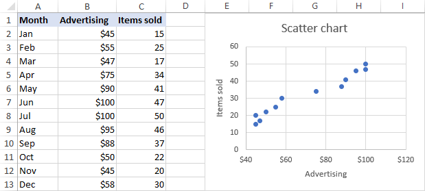
How can I add data labels from a third column to a scatterplot? Do you want to add data labels to the 3rd column values in the chart? Highlight the 3rd column range in the chart. Click the chart, and then click the Chart Layout tab. Under Labels, click Data Labels, and then in the upper part of the list, click the data label type that you want.

How to add data labels from different column in an Excel chart?
Best Types of Charts in Excel for Data Analysis, Presentation and ... 29/04/2022 · Learn to select best Excel Charts for Data Analysis, Presentation and Reporting within 15 minutes. ... #1 Use a bar chart whenever the axis labels are too long to fit in a column chart: ... the second category is ‘Feb’, the third category is ‘Mar’, etc. Data series – A data series is a set of related data points. Data points – A ...

Custom data labels in a chart
How to Use Cell Values for Excel Chart Labels - How-To Geek Select the chart, choose the "Chart Elements" option, click the "Data Labels" arrow, and then "More Options." Uncheck the "Value" box and check the "Value From Cells" box. Select cells C2:C6 to use for the data label range and then click the "OK" button. The values from these cells are now used for the chart data labels.

Create a Clustered AND Stacked column chart in Excel (easy)
Guide: How to Name Column in Excel | Indeed.com Select "Define Name" under the Defined Names group in the Ribbon to open the New Name window. Enter your new column name in the text box. Click the "Scope" drop-down menu and then "Workbook" to apply the change to all the sheets. 5. Clean all column names.

Combination Clustered and Stacked Column Chart in Excel ...
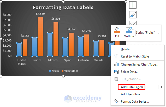
Adding rich data labels to charts in Excel 2013 | Microsoft 365 Blog One familiar and simple way is just single click on any data value (or column, in this example) to select the entire data series that it belongs to. Above, I have clicked all of the blue columns. Once the series is selected, I can right-click any column to pull up the context menu, then click the Add Data Labels entry.

How to add data labels from different column in an Excel chart?
Chart Data Labels > Alignment > Label Position: Outsid Despite this, the two sub-types behave differently. In the column chart, select the series. Go to the Chart menu > Chart Type. Verify the sub-type. If it's stacked column (the option in the first row that is second from the left), this is why Outside End is not an option for label position.

Apply Custom Data Labels to Charted Points - Peltier Tech
Analyze Data in Excel - support.microsoft.com Analyze Data in Excel empowers you to understand your data through high-level visual summaries, trends, and patterns. Simply click a cell in a data range, and then click the Analyze Data button on the Home tab. Analyze Data in Excel will analyze your data, and return interesting visuals about it in a task pane.

Change the format of data labels in a chart
How to Print Labels From Excel - EDUCBA Step #4 - Connect Worksheet to the Labels. Now, let us connect the worksheet, which actually is containing the labels data, to these labels and then print it up. Go to Mailing tab > Select Recipients (appears under Start Mail Merge group)> Use an Existing List. A new Select Data Source window will pop up.
How to Add Data Labels in Excel (2 Handy Ways) - ExcelDemy
Column Chart with Primary and Secondary Axes - Peltier Tech 28/10/2013 · The second chart shows the plotted data for the X axis (column B) and data for the the two secondary series (blank and secondary, in columns E & F). I’ve added data labels above the bars with the series names, so you can see where the zero-height Blank bars are. The blanks in the first chart align with the bars in the second, and vice versa.

Custom Data Labels with Colors and Symbols in Excel Charts ...
FAQ | MATLAB Wiki | Fandom Back to top A cell is a flexible type of variable that can hold any type of variable. A cell array is simply an array of those cells. It's somewhat confusing so let's make an analogy. A cell is like a bucket. You can throw anything you want into the bucket: a string, an integer, a double, an array, a structure, even another cell array. Now let's say you have an array of buckets - an array of ...
Using the CONCAT function to create custom data labels for an ...
Can I add data labels from an unrelated column to a simple 2-D column ... I would like to add data labels to the vertical chart representations with values from a third column. I am trying to show how many input/data points were included for each displayed column percentage (height) on the chart. The third column values range from 10-200, with an couple outliers up to 5,500, so a third axis doesn't display the data well.
Labels on Excel Chart - Microsoft Community
Apply Custom Data Labels to Charted Points - Peltier Tech Click once on a label to select the series of labels. Click again on a label to select just that specific label. Double click on the label to highlight the text of the label, or just click once to insert the cursor into the existing text. Type the text you want to display in the label, and press the Enter key.

How to Create Multi-Category Chart in Excel - Excel Board
How to add data labels from different column in an Excel chart? This method will guide you to manually add a data label from a cell of different column at a time in an Excel chart. 1. Right click the data series in the chart, and select Add Data Labels > Add Data Labels from the context menu to add data labels. 2.

Apply Custom Data Labels to Charted Points - Peltier Tech
Advanced Excel - Data Model - tutorialspoint.com The existing database relationships between those tables is used to create the Data Model in Excel. Step 1 − Open a new blank Workbook in Excel. Step 2 − Click on the DATA tab. Step 3 − In the Get External Data group, click on the option From Access. The Select Data Source dialog box opens. Step 4 − Select Events.accdb, Events Access ...
How to Add Data Labels in Excel (2 Handy Ways) - ExcelDemy
Excel, giving data labels to only the top/bottom X% values 1) Create a data set next to your original series column with only the values you want labels for (again, this can be formula driven to only select the top / bottom n values). See column D below. 2) Add this data series to the chart and show the data labels. 3) Set the line color to No Line, so that it does not appear! 4) Volia! See Below! Share
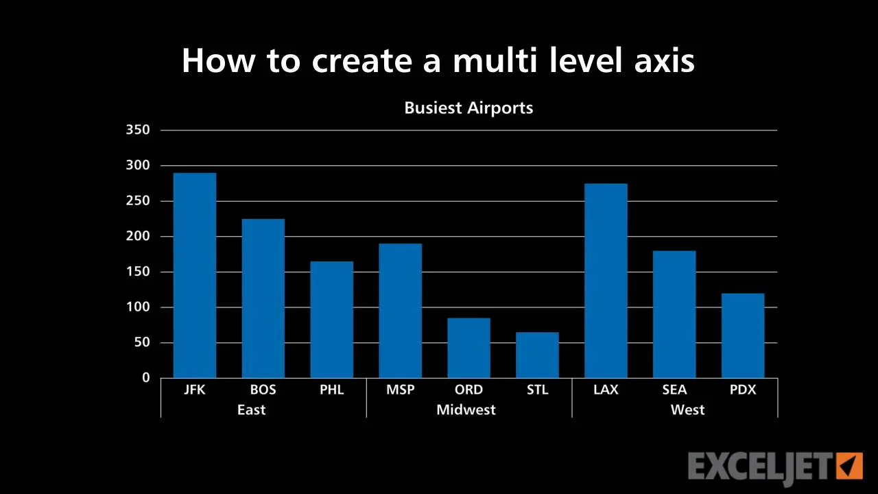
How to create a multi level axis
Prevent Overlapping Data Labels in Excel Charts - Peltier Tech Overlapping Data Labels. Data labels are terribly tedious to apply to slope charts, since these labels have to be positioned to the left of the first point and to the right of the last point of each series. This means the labels have to be tediously selected one by one, even to apply "standard" alignments.
Find, label and highlight a certain data point in Excel ...
Custom Excel Chart Label Positions • My Online Training Hub Custom Excel Chart Label Positions - Setup. The source data table has an extra column for the 'Label' which calculates the maximum of the Actual and Target: The formatting of the Label series is set to 'No fill' and 'No line' making it invisible in the chart, hence the name 'ghost series': The Label Series uses the 'Value ...

How to Add Total Data Labels to the Excel Stacked Bar Chart ...
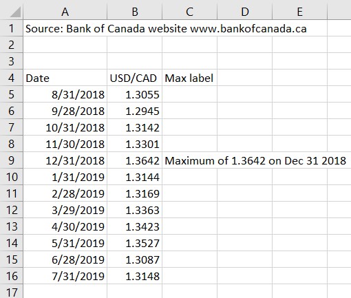
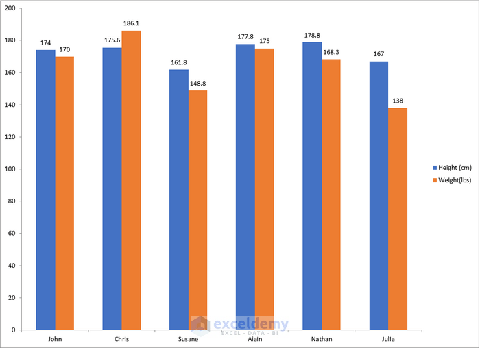
Using Data Labels from a Third Data Column in an Chart Excel 2013, allows you to select Data Labels locations from a Dialog box Prior to that it had to be done either manually or via a Macro To do it manually Select a Series Add a Data Label Select the Data Labels Then select an Individual Data Label In the formula bar =$D$2 (Cell reference to your new labels) Repeat for all Labels G guna_sekar87

Adding rich data labels to charts in Excel 2013 | Microsoft ...
How to Create Labels in Word from an Excel Spreadsheet - Online Tech Tips 12/07/2021 · 3. Bring the Excel Data Into the Word Document. Now that your labels are configured, import the data you saved in your Excel spreadsheet into your Word document. You don’t need to open Excel to do this. To start: While your Word document is still open, select the Mailings tab at the top.
How to Format Data Labels in Excel (with Easy Steps) - ExcelDemy
Excel Chart where data label moves to most recent data point Edit: I should have explained the expected data layout.The x values are in col. A starting with A2 (and A1 has a header). The y values are similarly organized in column B. Now, plot 2 series, the first with XVals and YVals, the 2nd with LastXVal and LastYVal.

Format Data Labels in Excel- Instructions - TeachUcomp, Inc.
How to show percentages in stacked column chart in Excel? - ExtendOffice 3. In Excel 2007, click Layout > Data Labels > Center . In Excel 2013 or the new version, click Design > Add Chart Element > Data Labels > Center. 4. Then go to a blank range and type cell contents as below screenshot shown: 5. Then in cell next to the column you type this =B2/B$6 (B2 is the cell value you want to show as percentage, B$6 is the ...
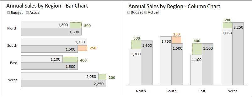
Actual vs Budget or Target Chart in Excel - Variance on ...
3 Axis Graph Excel Method: Add a Third Y-Axis - EngineerExcel Create a 3 Axis Graph in Excel. Scale the Data for an Excel Graph with 3 Variables. Decide on a Position for the Third Y-Axis. Select the Data for the 3 Axis Graph in Excel. Create Three Arrays for the 3-Axis Chart. How to Add a Third Axis in Excel: Create an "axis" from the fourth data series. Add Data Labels To a Multiple Y-Axis Excel Chart.

Apply Custom Data Labels to Charted Points - Peltier Tech

Custom data labels in a chart
How to Create a Graph with Multiple Lines in Excel | Pryor ...

Custom Data Labels with Colors and Symbols in Excel Charts ...

How to Customize for a GREAT-Looking Excel Chart

How to Add Data Labels to an Excel 2010 Chart - dummies

Excel: Clustered Column Chart with Percent of Month ...
EXCEL Charts: Column, Bar, Pie and Line

Add Labels ON Your Bars

Adding rich data labels to charts in Excel 2013 | Microsoft ...
How To Show Or Hide Data Labels On MS Excel? | My Windows Hub

Add or remove data labels in a chart
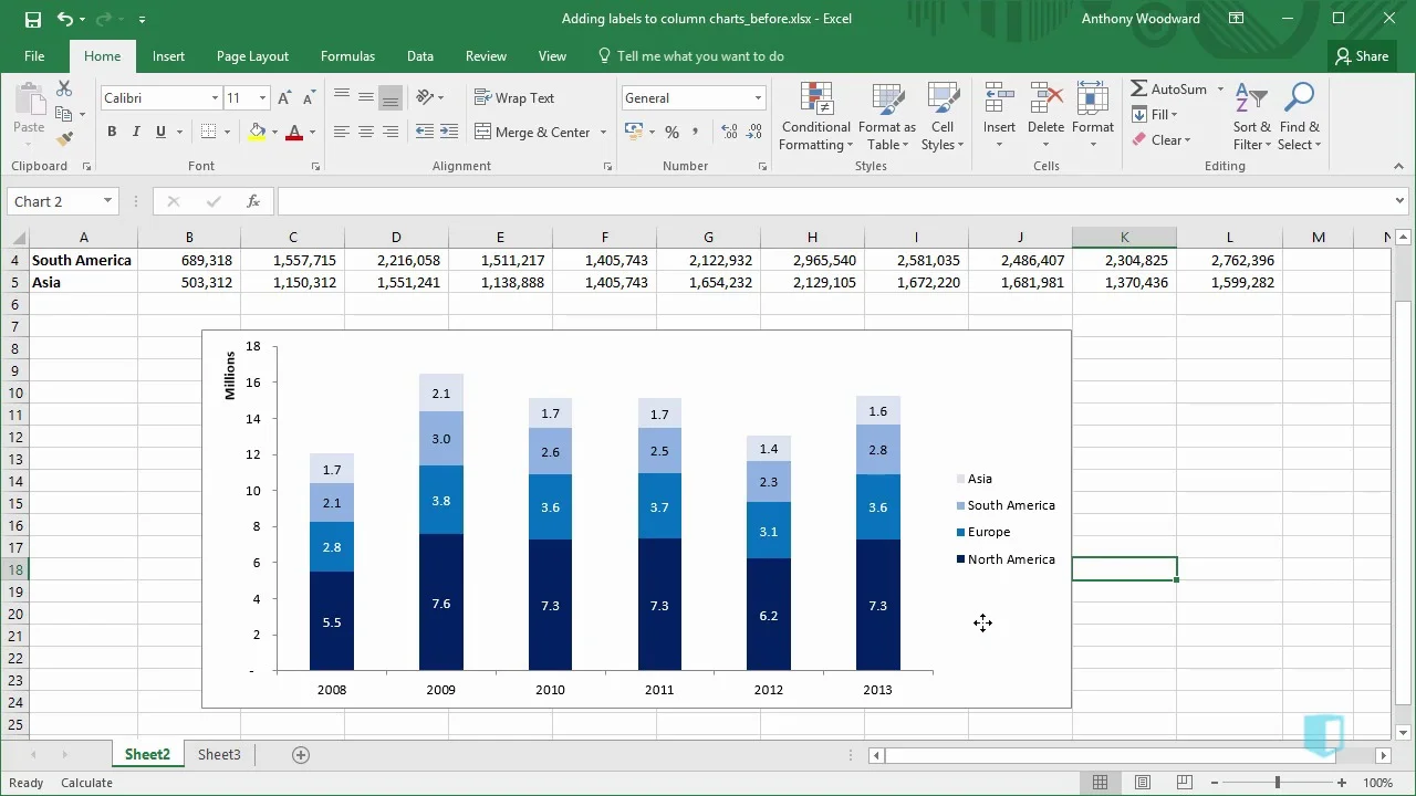
Adding Labels to Column Charts | Online Excel - KPMG Tax - Digital Now Course Training

Excel: Clustered Column Chart with Percent of Month ...
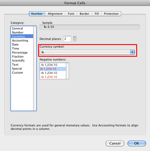
Format Number Options for Chart Data Labels in Excel 2011 for Mac

How to add total labels to stacked column chart in Excel?

How to add live total labels to graphs and charts in Excel ...

Excel VBA - Add Data Labels from Table body range - Stack ...

how to add data labels into Excel graphs — storytelling with data

How to show data labels in PowerPoint and place them ...

How to add live total labels to graphs and charts in Excel ...
Post a Comment for "43 excel data labels from third column"