45 how to format data labels in excel charts

Formatting Long Labels in Excel - PolicyViz Copy your graph Open PowerPoint and Paste the graph. Don't worry about the slide size or anything, just paste it in. Select the axis you want to format and select the Format option in the Paragraph menu. In the ensuing menu, select the Right option in the Alignment drop-down menu. How to: Display and Format Data Labels - DevExpress To apply a number format to data labels, utilize the DataLabelBase.NumberFormat property, which provides access to the NumberFormatOptions object containing format options for displaying numbers in different chart elements. Next, assign the corresponding number format code to the NumberFormatOptions.FormatCode property.

How to use cell values for excel chart labels - How to Note: The names of the tabs within Chart Tools differs depending on the version of Excel you are using. On the Format tab, in the Current Selection group, click the arrow next to the Chart Elements box, ... Use Cell Values for Chart Data Labels. Select range A1:B6 and click Insert > Insert Column or Bar Chart > Clustered Column. ...

How to format data labels in excel charts

Modifying Axis Scale Labels (Microsoft Excel) Follow these steps: Create your chart as you normally would. Double-click the axis you want to scale. You should see the Format Axis dialog box. (If double-clicking doesn't work, right-click the axis and choose Format Axis from the resulting Context menu.) Make sure the Number tab is displayed. (See Figure 1.) How to Create and Customize a Treemap Chart in Microsoft Excel Either right-click the chart and pick "Format Chart Area" or double-click the chart to open the sidebar. On Windows, you'll see two handy buttons on the right of your chart when you select it. With these, you can add, remove, and reposition Chart Elements. And you can pick a style or color scheme with the Chart Styles button. How to format bar charts in Excel — storytelling with data 12.09.2021 · Another benefit of doing this is that now there’s enough space to pull the long data labels into the ends of the bars. This is just one of the decluttering steps we can take to reduce perceived cognitive burden. Here’s how to achieve this: 3. Click on any data label to highlight them all, then right-click and choose Format Data Labels:

How to format data labels in excel charts. How to rename a data series in microsoft excel - How to To format data labels in Excel, choose the set of data labels to format. To do this, click the "Format" tab within the "Chart Tools" contextual tab in the Ribbon. Then select the data labels to format from the "Chart Elements" drop-down in the "Current Selection" button group. Create Dynamic Chart Data Labels with Slicers - Excel Campus 10.02.2016 · Step 3: Use the TEXT Function to Format the Labels. Typically a chart will display data labels based on the underlying source data for the chart. In Excel 2013 a new feature called “Value from Cells” was introduced. This feature allows us to specify the a range that we want to use for the labels. excel - Formatting Data Labels on a Chart - Stack Overflow sub charttest () activesheet.chartobjects ("chart 6").activate z = 1 with activechart if .charttype = xlline then i = .seriescollection (1).points.count activechart.fullseriescollection (1).datalabels.select for pts = 1 to i activechart.fullseriescollection (1).points (pts).hasdatalabel = true ' make sure all points are visible data … How to Print Labels from Excel - Lifewire Choose Start Mail Merge > Labels . Choose the brand in the Label Vendors box and then choose the product number, which is listed on the label package. You can also select New Label if you want to enter custom label dimensions. Click OK when you are ready to proceed. Connect the Worksheet to the Labels

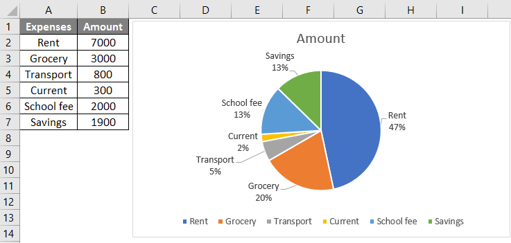
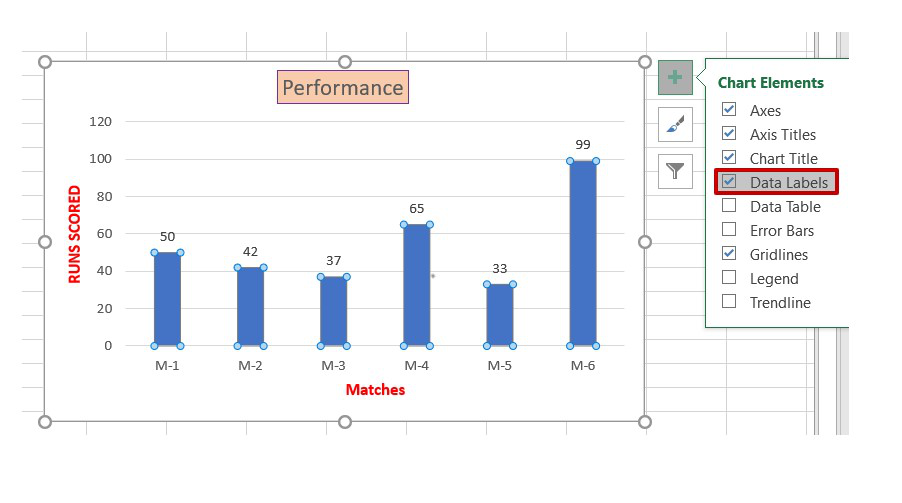
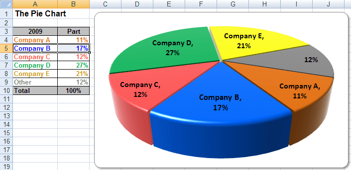
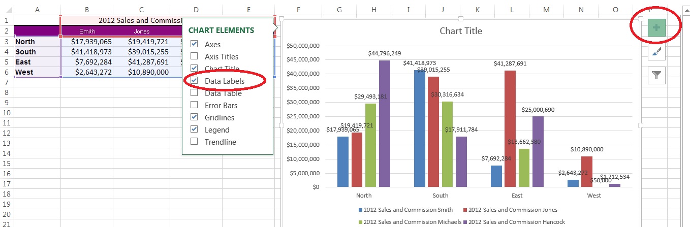
How to Change Excel Chart Data Labels to Custom Values? 05.05.2010 · Now, click on any data label. This will select “all” data labels. Now click once again. At this point excel will select only one data label. Go to Formula bar, press = and point to the cell where the data label for that chart data point is defined. Repeat the process for all other data labels, one after another. See the screencast. Step-by-Step Guide on How to Make a Chart in Excel (And Tips) Here's a list of the step-by-step process for how to make a chart in Excel: 1. Create your spreadsheet. First, open the spreadsheet with the relevant data you want to put in the chart or graph. If you don't have an existing document, you can create a new spreadsheet and manually input the data. Change the format of data labels in a chart Data labels make a chart easier to understand because they show details about a data series or its individual data points. For example, in the pie chart below, without the data labels it would be difficult to tell that coffee was 38% of total sales. You can format the labels to show specific labels elements like, the percentages, series name, or category name. › charts › dynamic-chart-dataCreate Dynamic Chart Data Labels with Slicers - Excel Campus Feb 10, 2016 · Step 3: Use the TEXT Function to Format the Labels. Typically a chart will display data labels based on the underlying source data for the chart. In Excel 2013 a new feature called “Value from Cells” was introduced. This feature allows us to specify the a range that we want to use for the labels.

DataLabels object (Excel) | Microsoft Docs Copy With Charts (1).SeriesCollection (1) .HasDataLabels = True .DataLabels.NumberFormat = "##.##" End With Use DataLabels ( index ), where index is the data-label index number, to return a single DataLabel object. The following example sets the number format for the fifth data label in series one in embedded chart one on worksheet one. VB Copy chandoo.org › wp › change-data-labels-in-chartsHow to Change Excel Chart Data Labels to Custom Values? May 05, 2010 · Now, click on any data label. This will select “all” data labels. Now click once again. At this point excel will select only one data label. Go to Formula bar, press = and point to the cell where the data label for that chart data point is defined. Repeat the process for all other data labels, one after another. See the screencast. › products › powerpointFormat Number Options for Chart Data Labels in PowerPoint ... Oct 21, 2013 · Alternatively, select the Data Labels for a Data Series in your chart and right-click (Ctrl+click) to bring up a contextual menu -- from this menu, choose the Format Data Labels option as shown in Figure 3. Figure 3: Select the Format Data Labels option Either of the above options will summon the Format Data Labels dialog box -- make sure that ... How to Create a Run Chart in Excel (2021 Guide) | 2 Free Templates Go to the Insert tab. Click " Insert Line or Area Chart .". Choose " Line .". You now have your simple run chart as a result: Step 3. Spruce Up Your Run Chart. Technically, you're good to go, but if you're looking to improve your chart from boring to beautiful in mere moments, here's how you can quickly spruce it up.

Excel Chart Elements: Parts of Charts in Excel | ExcelDemy

How to Find, Highlight, and Label a Data Point in Excel Scatter Plot? By default, the data labels are the y-coordinates. Step 3: Right-click on any of the data labels. A drop-down appears. Click on the Format Data Labels… option. Step 4: Format Data Labels dialogue box appears. Under the Label Options, check the box Value from Cells . Step 5: Data Label Range dialogue-box appears.

Data Driven Polar Charts for PowerPoint - SlideModel

Custom Chart Data Labels In Excel With Formulas Follow the steps below to create the custom data labels. Select the chart label you want to change. In the formula-bar hit = (equals), select the cell reference containing your chart label's data. In this case, the first label is in cell E2. Finally, repeat for all your chart laebls.

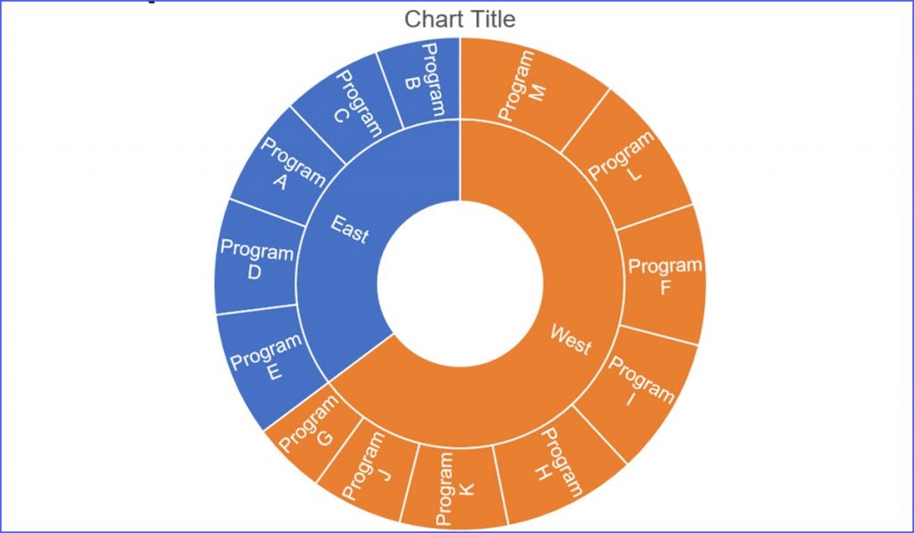
How to Create Multi-Category Chart in Excel - Excel Board

How to make a quadrant chart using Excel - Basic Excel Tutorial Format data labels. Right-click on any label and select 'Format Data Labels.' Go to the 'Label Options' tab and check the 'Value from cells' option. Select all the names and click OK. Uncheck the 'Y Value' box and under 'Label Position,' select 'Above. 7. Add the Axis titles.

Excel Charts: Creating Custom Data Labels - YouTube

Chart.ApplyDataLabels method (Excel) | Microsoft Docs ApplyDataLabels ( Type, LegendKey, AutoText, HasLeaderLines, ShowSeriesName, ShowCategoryName, ShowValue, ShowPercentage, ShowBubbleSize, Separator) expression A variable that represents a Chart object. Parameters Example This example applies category labels to series one on Chart1. VB Copy Charts ("Chart1").SeriesCollection (1).

Microsoft Tips with Temo!: How to Add Data Labels to an Excel 2010 Chart

› blog › 2021/9/8How to format bar charts in Excel — storytelling with data Sep 12, 2021 · Another benefit of doing this is that now there’s enough space to pull the long data labels into the ends of the bars. This is just one of the decluttering steps we can take to reduce perceived cognitive burden. Here’s how to achieve this: 3. Click on any data label to highlight them all, then right-click and choose Format Data Labels:

Enable or Disable Excel Data Labels at the click of a button - How To - PakAccountants.com

peltiertech.com › prevent-overlapping-data-labelsPrevent Overlapping Data Labels in Excel Charts - Peltier Tech May 24, 2021 · Overlapping Data Labels. Data labels are terribly tedious to apply to slope charts, since these labels have to be positioned to the left of the first point and to the right of the last point of each series. This means the labels have to be tediously selected one by one, even to apply “standard” alignments.

Pie Chart Examples | Types of Pie Charts in Excel with Examples

How to Make a Pie Chart in Excel & Add Rich Data Labels to The Chart! 7) With the data point still selected, go to Chart Tools>Format>Shape Styles and click on the drop-down arrow next to Shape Effects and select Shadow and choose Inner Shadow>Inside Diagonal Top Left. 8) With the one data point still selected, right-click this data point, and select Add Data Label>Add Data Callout as shown below.

How to Add Data Labels in Excel - Excelchat | Excelchat

Prevent Overlapping Data Labels in Excel Charts - Peltier Tech 24.05.2021 · Overlapping Data Labels. Data labels are terribly tedious to apply to slope charts, since these labels have to be positioned to the left of the first point and to the right of the last point of each series. This means the labels have to be tediously selected one by one, even to apply “standard” alignments.

Surface Chart in Excel

How To Add Data Labels In Excel | Independencereferendum 2022 On the chart tools layout tab, click the data labels button in the labels group. It may be in a folder called microsoft office. Click any data label to select all data labels, and then click the specified data label to. Excel Provides Several Options For The Placement And Formatting Of Data Labels. This will select "all" data labels.

How to Make a Sunburst Chart - ExcelNotes

Adding Colored Regions to Excel Charts - Duke Libraries Center for Data ... 12.11.2012 · Time series data is easy to display as a line chart, but drawing an interesting story out of the data may be difficult without additional description or clever labeling. One option, however, is to add regions to your time series charts to indicate historical periods or visualization binary data. Here is an example where a … Continue reading Adding Colored Regions to …

Formatting Charts in Excel - GeeksforGeeks

Format Chart Axis in Excel - Axis Options However, In this blog, we will be working with Axis options, Tick marks, Labels, Number > Axis options> Axis options> Format Axis Pane. Axis Options: Axis Options There are multiple options So we will perform one by one. Changing Maximum and Minimum Bounds The first option is to adjust the maximum and minimum bounds for the axis.

Custom Data Labels with Colors and Symbols in Excel Charts – [How To] - KING OF EXCEL

Differences between the OpenDocument Spreadsheet (.ods) format … Charts. Data labels. Not Supported. When you open an .ods format file in Excel for the web, some Data Labels are not supported. Charts. Shapes on charts. Partially supported. When you save the file in .ods format and open it again in Excel, some Shape types are not supported. Charts. Data tables. Not Supported. Charts. Drop Lines. Not Supported ...

Excel 3-D Pie charts - Microsoft Excel 2016

support.microsoft.com › en-us › officeChange the format of data labels in a chart To get there, after adding your data labels, select the data label to format, and then click Chart Elements > Data Labels > More Options. To go to the appropriate area, click one of the four icons ( Fill & Line , Effects , Size & Properties ( Layout & Properties in Outlook or Word), or Label Options ) shown here.

Excel 3-D Pie Charts

How to Show Percentage in Excel Pie Chart (3 Ways) We can open the Format Data Labels window in the following two ways. 2.1 Using Chart Elements. To active the Format Data Labels window, follow the simple steps below. Steps: Click on the pie chart to make it active. Now, click the Chart Elements button ( the Plus + sign at the top right corner of the pie chart). Click the Data Labels checkbox ...

Excel Course: Inserting Graphs

Pie Chart in Excel - Inserting, Formatting, Filters, Data Labels Right click on the Data Labels on the chart. Click on Format Data Labels option. Consequently, this will open up the Format Data Labels pane on the right of the excel worksheet. Mark the Category Name, Percentage and Legend Key. Also mark the labels position at Outside End. This is how the chark looks. Formatting the Chart Background, Chart Styles

Quick Tip: Excel 2013 offers flexible data labels - TechRepublic

How to add data labels from different column in an Excel chart? This method will introduce a solution to add all data labels from a different column in an Excel chart at the same time. Please do as follows: 1. Right click the data series in the chart, and select Add Data Labels > Add Data Labels from the context menu to add data labels. 2. Right click the data series, and select Format Data Labels from the ...

31 What Is A Label In Excel - Labels For Your Ideas

Change the Font Size, Color, and Style of an Excel Form Control Label In fact, whatever formatting exists in the cell when you first make the link, the label will maintain this format until a new link is created. For example, if I were to change G2 to a black color and a smaller font, the label would not show these new changes (however, it would change its text if I changed the value in G2 to something else).

Share :