41 how to add axis labels in excel 2013

Add axis label in excel | WPS Office Academy 1. First click so you can choose the type of chart where you want to place the axis label. 2. Now click where the chart elements button is located in the right corner of the chart. Then where the expanded menu is located, you must mark the axis titles alternative. 3. Excel tutorial: How to customize axis labels Instead you'll need to open up the Select Data window. Here you'll see the horizontal axis labels listed on the right. Click the edit button to access the label range. It's not obvious, but you can type arbitrary labels separated with commas in this field. So I can just enter A through F. When I click OK, the chart is updated.

Excel 2013 - Chart loses axis labels when grouping (hiden) values 3) Make sure you have Sunday and Monday displayed as labels. 4) Select columns A and B, go to Data => Group => Columns (the table will be hidden and the graph will appear with no data) 5) Save che workbook and close it. 6) Open the workbook and click the (+) sign to show the hiden columns. 7) you'll notice that axis labels (Sunday, Monday) are ...

How to add axis labels in excel 2013

Change axis labels in a chart - support.microsoft.com Right-click the category labels you want to change, and click Select Data. In the Horizontal (Category) Axis Labels box, click Edit. In the Axis label range box, enter the labels you want to use, separated by commas. For example, type Quarter 1,Quarter 2,Quarter 3,Quarter 4. Change the format of text and numbers in labels How to Add Axis Labels in Microsoft Excel - Appuals.com Click anywhere on the chart you want to add axis labels to. Click on the Chart Elements button (represented by a green + sign) next to the upper-right corner of the selected chart. Enable Axis Titles by checking the checkbox located directly beside the Axis Titles option. How to Add Axis Titles in a Microsoft Excel Chart Select your chart and then head to the Chart Design tab that displays. Click the Add Chart Element drop-down arrow and move your cursor to Axis Titles. In the pop-out menu, select "Primary Horizontal," "Primary Vertical," or both. If you're using Excel on Windows, you can also use the Chart Elements icon on the right of the chart.

How to add axis labels in excel 2013. How to Add Axis Labels in Excel 2013 - YouTube This is a tutorial on how to add axis labels in Excel 2013. Axis labels, for the most part, are added immediately to your chart once it is created. in Excel 2013, when the chart is highlighted, you... How to Add Axis Labels in Excel Charts - Step-by-Step (2022) How to add axis titles 1. Left-click the Excel chart. 2. Click the plus button in the upper right corner of the chart. 3. Click Axis Titles to put a checkmark in the axis title checkbox. This will display axis titles. 4. Click the added axis title text box to write your axis label. Excel Chart Vertical Axis Text Labels - My Online Training Hub Excel 2010: Chart Tools: Layout Tab > Axes > Secondary Vertical Axis > Show default axis. Excel 2013: Chart Tools: Design Tab > Add Chart Element > Axes > Secondary Vertical. Now your chart should look something like this with an axis on every side: Click on the top horizontal axis and delete it. While you're there set the Minimum to 0, the ... How to add axis label to chart in Excel? - ExtendOffice Add axis label to chart in Excel 2013. In Excel 2013, you should do as this: 1. Click to select the chart that you want to insert axis label. 2. Then click the Charts Elements button located the upper-right corner of the chart. In the expanded menu, check Axis Titles option, see screenshot: 3. And both the horizontal and vertical axis text boxes have been added to the chart, then click each of the axis text boxes and enter your own axis labels for X axis and Y axis separately.

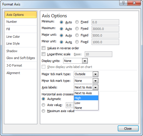
Excel tutorial: How to create a multi level axis To straighten out the labels, I need to restructure the data. First, I'll sort by region and then by activity. Next, I'll remove the extra, unneeded entries from the region column. The goal is to create an outline that reflects what you want to see in the axis labels. Now you can see we have a multi level category axis. Excel charts: add title, customize chart axis, legend and data labels Click anywhere within your Excel chart, then click the Chart Elements button and check the Axis Titles box. If you want to display the title only for one axis, either horizontal or vertical, click the arrow next to Axis Titles and clear one of the boxes: Click the axis title box on the chart, and type the text. Change axis labels in a chart in Office - support.microsoft.com In charts, axis labels are shown below the horizontal (also known as category) axis, next to the vertical (also known as value) axis, and, in a 3-D chart, next to the depth axis. The chart uses text from your source data for axis labels. To change the label, you can change the text in the source data. Changing Axis Labels in PowerPoint 2013 for Windows Make sure you then deselect everything in the chart, and then carefully right-click on the value axis. Figure 2: Format Axis option selected for the value axis This step opens the Format Axis Task Pane, as shown in Figure 3, below. Make sure that the Axis Options button is selected as shown highlighted in red within Figure 3.

How to Add a Secondary Axis in Excel Charts (Easy Guide) Below are the steps to add a secondary axis to the chart manually: Select the data set. Click the Insert tab. In the Charts group, click on the Insert Columns or Bar chart option. Click the Clustered Column option. In the resulting chart, select the profit margin bars. How to Create a Pareto Chart in Excel - Automate Excel Step #2: Add data labels. Start with adding data labels to the chart. Right-click on any of the columns and select "Add Data Labels." Customize the color, font, and size of the labels to help them stand out (Home > Font). Step #3: Add the axis titles. As icing on the cake, axis titles provide additional context to what the chart is all about. How To Add Axis Labels In Excel - BSUPERIOR To add the axes titles for your chart, follow these steps: Click on the chart area. Go to the Design tab from the ribbon. Click on the Add Chart Element option from the Chart Layout group. Select the Axis Titles from the menu. Select the Primary Vertical to add labels to the vertical axis, and Select the Primary Horizontal to add labels to the horizontal axis. Picture 1- Add axis title by the Add Chart Element option How to add secondary axis in Excel (2 easy ways) - ExcelDemy 2) Now right click on the Data Series and choose the Format Data Series option from the menu. 3) Format Data Series task pane appears on the right side of the worksheet. And we choose the Secondary Axis radio button for this data series. The keyboard shortcut to open this task pane is: CTRL + 1.

How to Insert Chart Axis Title in Excel 2010 - Ethical Hacking

How to Insert Axis Labels In An Excel Chart | Excelchat How to add vertical axis labels in Excel 2016/2013 We will again click on the chart to turn on the Chart Design tab We will go to Chart Design and select Add Chart Element Figure 6 - Insert axis labels in Excel In the drop-down menu, we will click on Axis Titles, and subsequently, select Primary vertical

Cascade Chart Creator for Microsoft Excel

How to Label Axes in Excel: 6 Steps (with Pictures) - wikiHow Steps Download Article 1 Open your Excel document. Double-click an Excel document that contains a graph. If you haven't yet created the document, open Excel and click Blank workbook, then create your graph before continuing. 2 Select the graph. Click your graph to select it. 3 Click +. It's to the right of the top-right corner of the graph.

Excel: axis label insert - here's how

Adjusting the Angle of Axis Labels (Microsoft Excel) Click the Format Axis option. Excel displays the Format Axis task pane at the right side of the screen. Click the Text Options link in the task pane. Excel changes the tools that appear just below the link. Click the Textbox tool. (It is the right-most tool in the task pane. It looks like a sheet of paper.)

How to change chart axis labels' font color and size in Excel?

Adding rich data labels to charts in Excel 2013 | Microsoft 365 Blog Putting a data label into a shape can add another type of visual emphasis. To add a data label in a shape, select the data point of interest, then right-click it to pull up the context menu. Click Add Data Label, then click Add Data Callout . The result is that your data label will appear in a graphical callout.

Changing Axis Labels in PowerPoint 2011 for Mac

Two-Level Axis Labels (Microsoft Excel) Put your second major group title into cell E1. In cells B2:G2 place your column labels. Select cells B1:D1 and click the Merge and Center tool. (In Excel 2007 the Merge and Center tool is in the Alignment group of the Home tab on the ribbon.) The first major group title should now be centered over the first group of column labels.

Combining several charts into one chart - Microsoft Excel 2010

Excel: Labeling Sparklines - Excel Articles Type each month letter separated by a space. Make the font as small as possible. Center the values. Make the column width wider until the labels line up with the chart. Use the labels around the sparkline to add labels. In the figure to the right, a formula calculates the max and min of each series. The REPT (CHAR (10),4) adds four line feeds.

r - Multi-row x-axis labels in ggplot line chart - Stack Overflow

How to Add a Axis Title to an Existing Chart in Excel 2013 Watch this video to learn how to add an axis title to your chart in Excel 2013. A chart has at least 2 axis: the horizontal x-axis ...

Share :