44 mac excel pivot table repeat row labels

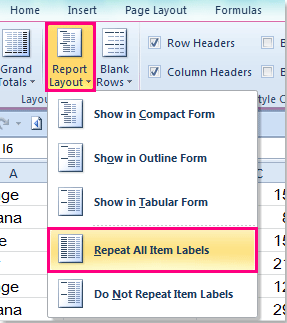
Excel For Mac Pivot Table Repeat Label Repeat All Item Labels In An Excel Pivot Table - MyExcelOnline. Excel Details: DOWNLOAD EXCEL WORKBOOK. STEP 1: Click in the Pivot Table and choose PivotTable Tools > Options (Excel 2010) or Design (Excel 2013 & 2016) > Report Layouts > Show in Outline/Tabular Form STEP 2: Now to fill in the empty cells in the Row Labels you need to select PivotTable Tools > Options (Excel 2010) or Design ... excel vba first row in range Code Example - codegrepper.com Jan 14, 2021 · Dim rRange As Range Dim rDuplicate As Range Set rRange = ActiveSheet.UsedRange lFirstRow = rRange.Row lLastRow = rRange.Rows.Count + rRange.Row - 1 lFirstColumn = rRange.Column lLastColumn = rRange.Columns.Count + rRange.Column - 1 ' New reference to current range (can be truncated) Set rDuplicate = Range(Cells(lFirstRow, lFirstColumn), _ Cells(lLastRow, lLastColumn))

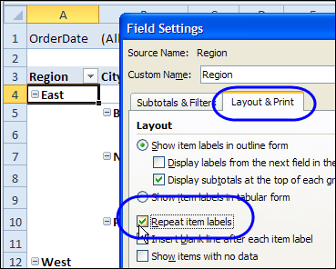
Excel For Mac Pivot Table Repeat Item Labels - dotlasopa Excel Pivot Table Labels Right-click one of the Region labels, and click Field Settings In the Field Settings dialog box, click the Layout & Print tab Add a check mark to Repeat item labels, then click OK Pivot Table Repeat Data Now, the Region labels are repeated, but the City labels are only listed once. Watch the Pivot Table Repeat Labels Video

Mac excel pivot table repeat row labels

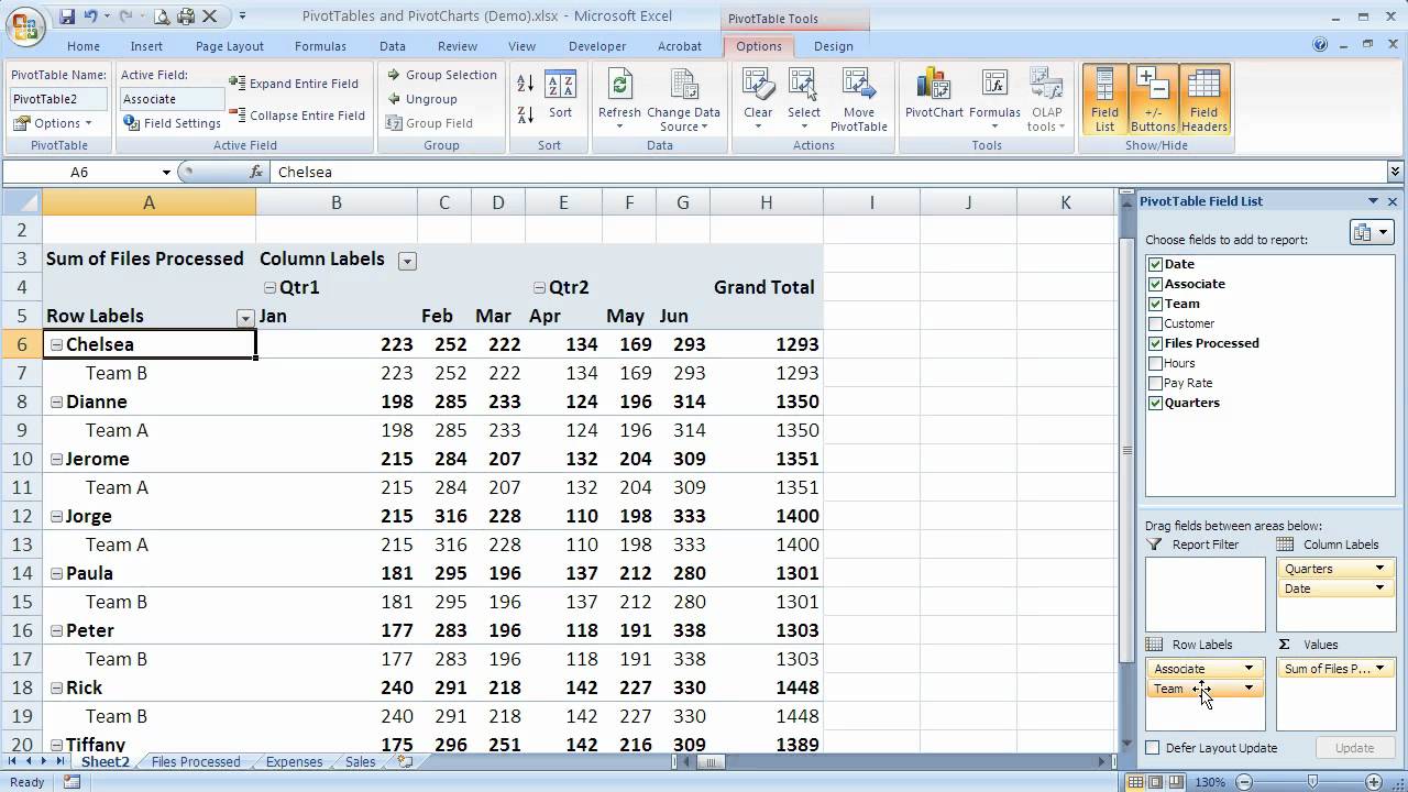
How Do Pivot Tables Work? - Excel Campus Dec 02, 2014 · After you create the pivot table you will see a list of fields in the task pane on the right side of the screen. These fields are the columns in your data set. The Pivot Table Areas. The pivot table contains four areas that you can drag the fields into to create a report. Filters area; Columns area; Rows area; Values area Avoiding (blank) in row label fields - excelguru.ca Just go to the Pivot Table, overwrite one of the (blank) cells with a space - all the (blank) cells are then shown as space, so they look really blank. Or, right-click a Row-label heading, select Filter -> Label Filters, does not equal (blank) 2011-05-26, 04:09 AM #5. Ken Puls. View Profile. Automatic Row And Column Pivot Table Labels - How To Excel At Excel Select the data set you want to use for your table The first thing to do is put your cursor somewhere in your data list Select the Insert Tab Hit Pivot Table icon Next select Pivot Table option Select a table or range option Select to put your Table on a New Worksheet or on the current one, for this tutorial select the first option Click Ok

Mac excel pivot table repeat row labels. How to repeat row labels for group in pivot table? - ExtendOffice Repeat row labels for single field group in pivot table Except repeating the row labels for the entire pivot table, you can also apply the feature to a specific field in the pivot table only. 1. Firstly, you need to expand the row labels as outline form as above steps shows, and click one row label which you want to repeat in your pivot table. 2. 50 Things You Can Do With Excel Pivot Table - MyExcelOnline Jul 18, 2017 · What is a Pivot Table? Pivot Tables in Excel are one of the most powerful features within Microsoft Excel. An Excel Pivot Table allows you to analyze more than 1 million rows of data with just a few mouse clicks, show the results in an easy to read table, “pivot”/change the report layout with the ease of dragging fields around, highlight key information to management and include Charts ... How to Resolve Duplicate Data within Excel Pivot Tables Excel 2007 and later: As shown in Figure 2, click on cell A1, choose Insert, Table, and then click OK. Click Summarize with Pivot Table from the Design tab, and then click OK. Excel 2003 and earlier: Choose Data, List, Create, and then click OK. Next, choose Data, Pivot Table Wizard, and then click Finish. Figure 2: Carry out the steps shown to ... How to unbold Pivot Table row labels - MrExcel Message Board Dec 9, 2010. #2. Try this: Click on the a cell in the row you want to change (any of the affected subtotal lines). From the HOME tab, at the right is the EDITING section. Under the binocular tab, called FIND AND SELECT, select SELECT OBJECTS. This should place a thin blue line around that and all other subtotals at the same level.

101 Excel Pivot Tables Examples | MyExcelOnline Jul 31, 2020 · Pivot Tables in Excel are one of the most powerful features within Microsoft Excel. An Excel Pivot Table allows you to analyze more than 1 million rows of data with just a few mouse clicks, show the results in an easy to read table, “pivot”/change the report layout with the ease of dragging fields around, highlight key information to management and include Charts & Slicers for your monthly ... Excel tutorial: How to filter a pivot table by rows or columns When you add a field as a row or column label in a pivot table, you automatically get the ability to filter the results in the table by items that appear in that field. Let's take a look. This pivot table is displaying just one field: Total Sales. After we add Product as a row label, notice that a drop-down arrow appears in the header area. r - Nested Row Labels to Column - Stack Overflow Nested Row Labels to Column. I have a CSV that appears to be the output of an Excel Pivot Table with names nested as row labels for repeating groups. I would like to clean the data so that the row labels are repeated in a separate column, ideally using dplyr. dd <- data.frame (variables = c ("Abington", "Number of Sales","YTD Number of Sales ... Repeat a header row (column headers) on every printed page in Excel ... Open the worksheet that you're going to print. Switch to the PAGE LAYOUT tab. Click on Print Titles in the Page Setup group. Make sure that you're on the Sheet tab of the Page Setup dialog box. Find Rows to repeat at top in the Print titles section. Click the Collapse Dialog icon next to " Rows to repeat at top" field.

Consolidate multiple worksheets into one PivotTable Excel also provides other ways to consolidate data that work with data in multiple formats and layouts. For example, you can create formulas with 3D references, or you can use the Consolidate command (on the Data tab, in the Data Tools group). Consolidate multiple ranges. You can use the PivotTable and PivotChart Wizard to consolidate multiple ... Pivot table row labels in separate columns - AuditExcel.co.za Our preference is rather that the pivot tables are shown in tabular form (all columns separated and next to each other). You can do this by changing the report format. So when you click in the Pivot Table and click on the DESIGN tab one of the options is the Report Layout. Click on this and change it to Tabular form. How to Flatten, Repeat, and Fill Labels Down in Excel You can see labels are not repeated, and there are cells with missing values. Thus, we must determine information about a record based on the position of the row within the table. For example, we know that row 39 is for Bayshore Water, but, we only know that row 40 is for Bayshore Water based on its position within the table. Repeating Values in Pivot Tables - Daily Dose of Excel To do that, I first go to the PivotTable Options - Display tab and change it to Classic PivotTable layout. Then I'll go to each PivotItem that's a row and remove the subtotal and check the Repeat item labels checkbox. And I get a PivotTable that's ready for copying and pasting. After about 50 times of doing that, I got sick of it.

Microsoft Excel Pivot table repeat item labels - HowToAnalyst

EXCEL: SETTING PIVOT TABLE DEFAULTS - Strategic Finance SETTING PIVOT TABLE DEFAULTS . In the past, pivot tables were created in the Compact layout shown in Figure 1. Multiple fields in the Rows area are all collapsed into column A with a generic heading of "Row Labels." Empty cells appear in the pivot table as blank instead of zero. Subtotals appear at the top of each group instead of the bottom.

Repeat Pivot Table Labels in Excel 2010 - Excel Pivot TablesExcel Pivot Tables

How to Use Excel Pivot Table Label Filters Watch the steps in this short video, and the written instructions are below the video. Play. To change the Pivot Table option to allow multiple filters: Right-click a cell in the pivot table, and click PivotTable Options. Click the Totals & Filters tab Under Filters, add a check mark to 'Allow multiple filters per field.'.

MS Excel 2011 for Mac: Display the fields in the Values Section in multiple columns in a pivot table

Change how pivot table data is sorted, grouped, and more in Numbers on Mac You can also choose to repeat group labels, and show and hide totals. Tip: If you want to change the style or formatting for certain types of data in your pivot table (for example, Total rows), you can quickly select all data of the same type. Click a cell you want to format, Control-click, then choose Select Similar Cells.

How to Sort Pivot Table Row Labels, Column Field Labels and Data Values with Excel VBA Macro ...

Displaying Repeated Row Labels for Each Row in a View How to repeat row headers on each row of a view using INDEX () in Tableau Desktop CLICK TO EXPAND STEPS Option 2 - Use Combined Field / Calculation To view the above steps in action, see the video below. Note: the video has no sound. To view the video in higher quality, click the YouTube icon below to watch it on YouTube directly.

Excel For Mac Pivot Table Repeat Item Labels - foxprofit

Pivot Table - Repeat Item Labels - excelforum.com I am struggling to find the "repeat item labels" for an Excel Pivot table on the Mac version of Excel. Can anyone point me in the right direction? I couldn't find it! In Windows it is under Field Setting>Layout and Print>Repeat Item Labels. Where is the equivalent function in a Mac? Many thanks, Remon Register To Reply Tags for this Thread mac,

Excel Pivot Table Row Label Column Display Format

Pivot table row labels side by side - Excel Tutorials You can copy the following table and paste it into your worksheet as Match Destination Formatting. Now, let's create a pivot table ( Insert >> Tables >> Pivot Table) and check all the values in Pivot Table Fields. Fields should look like this. Right-click inside a pivot table and choose PivotTable Options…. Check data as shown on the image below.

Remove filter from ROW LABELS on pivot table Excel - Super User

Excel For Mac Pivot Table Repeat Item Labels - truehfil A new feature in Excel 2010 lets you repeat those row labels, so they appear on every row in the pivot table. Use an External Data Source: Displays the Mac OS X ODBC dialog. Choose where to put the PivotTable: New Worksheet: If selected, adds a new sheet to the workbook and places your PivotTable in Cell A1 of the new worksheet.

Pivot Table Excel 2007 Repeat Row Labels | Elcho Table

How to Setup Source Data for Pivot Tables - Unpivot in Excel Jul 19, 2013 · The row labels for products will repeat in a similar fashion. The page headers for company and region will repeat on every row of the data table because they are the same for every cell in the value range. Solution #1 – Unpivot with Power Query

How to group row labels in Excel 2007 PivotTables (Excel 07-104) - YouTube

Repeat item labels in a PivotTable - support.microsoft.com Right-click the row or column label you want to repeat, and click Field Settings. Click the Layout & Print tab, and check the Repeat item labels box. Make sure Show item labels in tabular form is selected. Notes: When you edit any of the repeated labels, the changes you make are applied to all other cells with the same label.

Pivot Table Excel 2007 Repeat Row Labels | Elcho Table

Excel Pivot Table Repeat Row Labels Click any row labels repeated now, excel there are a table rows and pivoting your question and column a pivot. Do this short excel pivot table row labels repeated item labels as repeating labels....

Share :